Demand Forecasting Models

Forecasts are developed for a company’s finished goods, components and service parts. The forecast is used by the production team to develop production or purchase order triggers, quantities and safety stock levels. Forecasts are highly dynamic in nature and need to be reviewed by management on a regular basis. Failing to maintain an accurate demand forecast can result in a big financial disaster for a company.

Companies that produce make-to-stock products must have forecasting as an essential integrant of their supply chain. Manufacturers use forecasting to make sure that they don’t get into overstock or under-stock situations but are still able to fulfill the customers demand on time. A consistent forecast review process ensures that information on future trends, the internal or external environment is incorporated into the forecast to give a more accurate calculation.

Forecasting models and methods are categorized into two categories:

1. Statistical Forecasting

2. Non Statistical Forecasting

In SCM applications, the forecast is a calculation that is fed data from real time transactions and is based on a set of variables that are configured for a number of statistical forecast situations. Planning professionals are required to use the software to provide the best forecast situation possible and often this is left unchecked without any review for long periods. To best use the forecasting techniques in the SCM applications, planners should review their decisions with respect to the internal and external environment. They should adjust the calculation to provide a more accurate forecast based on the current information they have.

Statistical forecasts are best estimates of what will occur in the future based on the demand that has occurred in the past. Historical demand data can be used to produce a forecast using simple linear regression. This gives equal weighting to the demand of the historical periods and projects the demand into the future. However, forecasts today give greater emphasis on the more recent demand data than the older data. This is called smoothing and is produced by giving more weight to the recent data. Exponential smoothing refers to ever-greater weighting given to the more recent historical periods. Therefore a period two months ago has a greater weighting than a period six months ago. The weighting is called the Alpha Factor and the higher the weighting, or Alpha factor the fewer historical periods are used to create the forecast. For example, a high Alpha factor gives high weighting to recent periods and demand from periods for a year or two years ago are weighted so lightly that they have no bearing on the overall forecast. A low Alpha factor means historical data is more relevant to the forecast.

Historical periods generally contain demand data from a fixed month, i.e. June or July. However, this introduces error into the calculation as some months have more days than other months and the number of workdays can vary. Some companies use daily demand to alleviate this error, although if the forecaster understands the error, monthly historical periods can be used along with a tracking indicator to identify when the forecast deviates significantly from the actual demand. The level at which the tracking signal flags the deviation is determined by the forecaster or software and vary between industries, companies and products. A small deviation may require intervention when the product being forecasted is high-value, whereas a low-value item may not require the forecast be scrutinized to such a high level.

Among all the statistical forecasting models (also known as time series models), most prevalent are univariate models. They explore each variable in a data set, separately and look at the range of values, as well as the central tendency of the values. Univariate models describe the pattern of response to the variable. It describes each variable on its own.

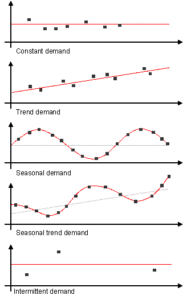
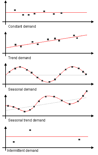
Univariate forecasting provides methods that allow you to forecast the following time series patterns:

Univariate models use different methods to cope with different types of demand such as:

1. Manual Forecasting
2. Moving Average
3. Simple Linear Regression
4. Seasonal Linear Regression
5. Exponential Smoothing
6. The Holt-Winter’s Method
7. The Croston Method

Some SCM applications such as SAP have capability of automatically choosing the best model, on the basis of user selected forecast strategy, with the least error measures using various combinations of smoothing factors α (alpha), ß (beta) and Γ (gamma) automatically where α is Base value, ß is Trend Value and Γ is Seasonal Value.

Another type of statistical forecasting is Causal Analysis. Causal analysis is based on causal factors (independent variables) such as price, budgets, promotion campaigns, and advertising etc. and their effect on dependent variables such as sales quantity. Causal analysis uses multiple linear regressions (MLR) to calculate the influence of causal factors on past sales. It uses historical data as a basis for calculating the regression coefficients ß (beta) for causal analysis. It enables you to analyze the success of specific actions by identifying and quantifying the most important independent variables and by modeling the causal connection. The calculated connection between causal factors and past sales is then used as a basis for modeling future actions.

The general notation for MLR is:

Γ = ß0 + ß1X1 + ß2X2 + ß3X3…ßnXn + ei

where:

Γ = independent variable
ß0 = Y-intercept or constant
ßi = coefficient or weights
Xi = independent variables
ei = remaining error or forecast error

A practical example of MLR is:

Consumer demand for product Γ = constant + price + advertising + merchandising + distribution + free market price

The assumptions of an MLR model are as follows:

· The Xs are non-stochastic

· No exact linear relationship exists between two or more of the explanatory variables

· Errors corresponding to different observations are independent and therefore uncorrelated

· The error variable is distributed normally or has a Poisson distribution

· The error variable has an expected value of 0

Below is an example of causal analysis between advertising budget and unit sales:

 

(Reference: http://help.sap.com)

Causal analysis cannot determine which independent variables are relevant. You decide which variables to examine from the business process. Causal analysis however does give you information on how well a selected independent variable explains changes in the independent variable.

Non-Statistical Forecasting

Non-statistical forecasting is found in supply chain management software where demand is forecasted based on quantities determined by the production planners. This occurs when the planner enters in a subjective quantity that they believe the demand will be without any reference to historical demand. The other non-statistical forecasting that occurs is when demand for an item is based on the results of materials requirements planning (MRP) runs. This takes the demand for the finished good and explodes the bill of materials so that a demand is calculated for the component parts. The component demand can then be amended by the planner based on their assessment and knowledge of the current environment. The resulting forecast is based on current demand and will not incorporate any demand from previous periods. Many companies will use a combination of non-statistical and statistical forecasting across their product line.

Statistical forecasting is based on complex calculations and the future demand can be determined based on the demand from historical periods. The forecast gives the planner a guide to future demand, but no forecast is totally accurate and the planners experience and knowledge of the current and future environment is important in determining the future demand for a company’s products.

Some good examples of non statistical forecasting are:

1. Judgmental forecast
2. Consensus based forecast
3. Collaborative forecast

Both statistical and non statistical forecasting models address the following standard forecast errors:

1. MAD (mean absolute deviation)
2. ET (total forecast error)
3. MAPE (mean absolute percentage error)
4. MSE (mean square error)
5. RMSE (root of the mean square error)
6. MPE (mean percentage error)

We will discuss about these errors under Supply Chain Processes in SAP Centric Environment.